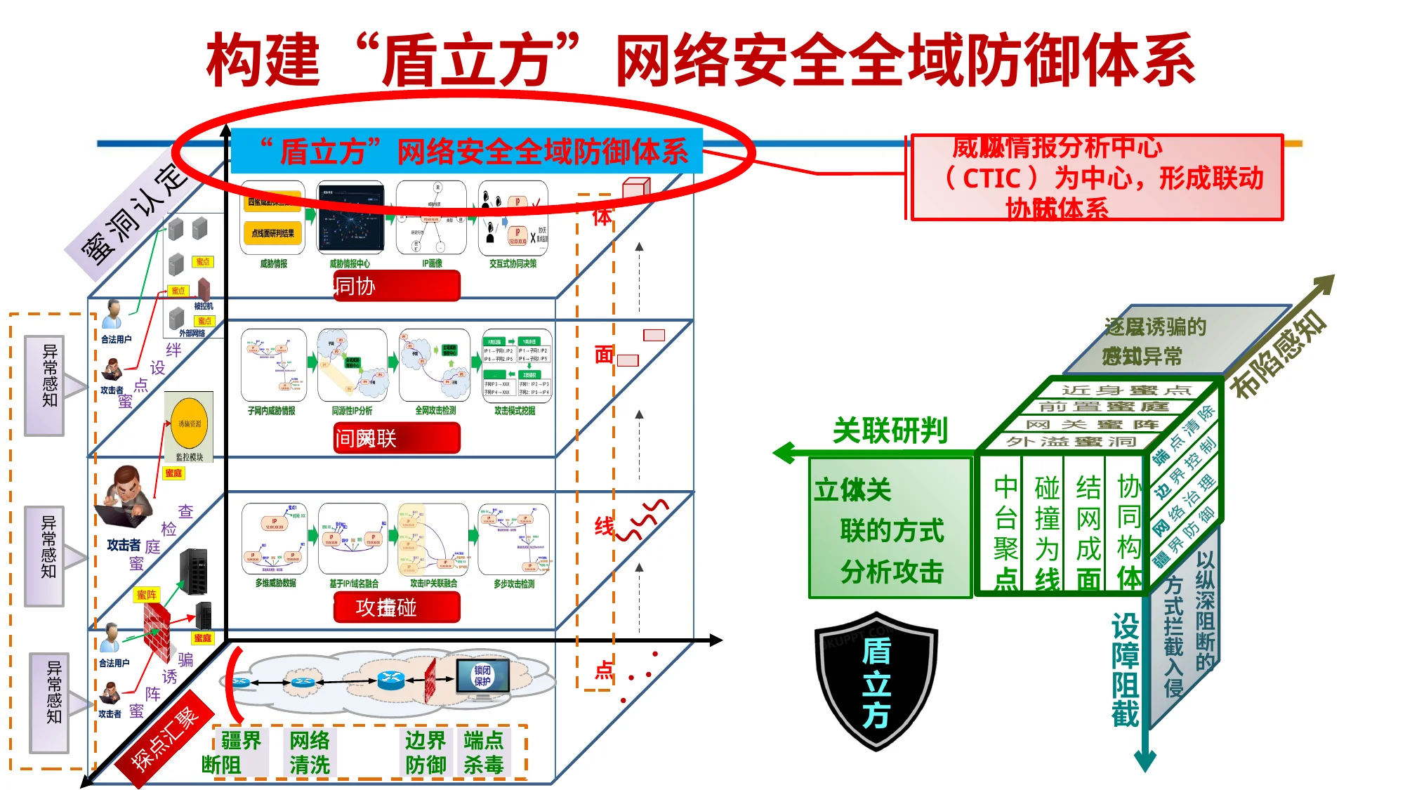
In September 2025, a large internal leak from Geedge Networks and MESA Lab appeared online: roughly 600GB from a security vendor and a prestigious research lab that builds China’s censorship technology. Most of it was code. Buried beside the code was the part I wanted: 54,761 documents of papers, student theses, and internal project files.

I don’t read Chinese. My Chinese comprehension is limited to random words like “correct horse battery staple”.

I built a pipeline to analyze those documents anyway. This post covers what it cost, what it got wrong, and what transfers to any CTI analyst staring at a document pile in a language they don’t read. This is the methodology that helped me write my DNS4CN piece.

TLDR; Subject-matter expertise still wins; verify everything else. Treat the model as a research assistant.

Manual triage does not scale

Basic egrep and sorting by file size surfaced some interesting things. But searching in English, by hand, across tens of thousands of files would have taken weeks. A tiny local stack using AnythingLLM and LM Studio choked on a few dozen files and would lie to me: no file citations, so no way to tell a real finding from a hallucination. The workflow turned into a labor-intensive version of copy/paste into Google Translate.

And there’s no economical way to put 65GB of documents in front of any model, local or frontier.

The fix was to change what I spent where. Spend cheap local compute on extracting, OCRing, and organizing every document. Spend expensive model attention on the handful most relevant to the topic.

Handling the material

Nothing exotic here, just standard practice for untrusted files. Early reporting warned that the leak might contain malware (I did not extract the Git repos, only documents), and the parsers this pipeline leans on (LibreOffice, poppler, exiftool) have a CVE history on malformed input. So the work ran in a dedicated WSL2 instance, the source directory stayed read-only, outbound network was limited to the two endpoints the pipeline needs, and I verified the torrent hash before trusting any file.

The shared foundation

Everything downstream reads from one corpus, built once in three stages.

flowchart TD
    SRC[("leak archives + loose docs
read-only, ~52GB")]

    subgraph CORPUS["Corpus build — runs once, topic-agnostic"]
        S1["Stage 1 · extract archives"]
        S2["Stage 2 · inventory"]
        S3["Stage 3 · extract text
unstructured + LibreOffice, resumable"]
        E3[("text/shard_*.jsonl
54,761 docs · 617MB")]
    end

    SRC --> S1 --> S2 --> S3 --> E3
    E3 --> WA["Workflow A: 
batch topic retrieval"]
    E3 --> WB["Workflow B: 
RAG semantic search"]

    class SRC,E3 store
    class S1,S2,S3 stage
    class WA,WB flow

Stage 1 extracts the archives. Straightforward: untar the *.tar.zst source archives. About 52GB of compressed archives become 65GB of extracted documents.

Stage 2 builds an inventory. A metadata catalog is faster than walking the filesystem every time I need to touch tens of thousands of files. It dedupes on modified time, detects each document’s language, records whether OCR supplied the text, and assigns every document a stable SHA1-derived ID that the later stages key off of.

Stage 3 extracts the text. This is where the token savings come from. Instead of shipping a 20MB PowerPoint to the model and making it do the parsing, I pull the text out first and keep only that. The model never sees office metadata, and it never has to run extraction tooling itself.

That sounds clean until you’re working across two languages, English and Mandarin, in documents that mix both with different fonts and encodings.

The first version of this stage used fast extraction with no OCR at all. That’s how it missed several key documents: PDFs with no text layer, photos someone had pasted into a document and saved (the pipeline missed the single most important document this way!). They extracted to nothing, scored zero, and disappeared before any model saw them. The fix was a second pass that re-extracts low-text documents with OCR, which is now part of the stage. Every stage builds on the one before it, and Stage 3 is the most important. Get extraction wrong and every later stage reasons over gaps it can’t see.

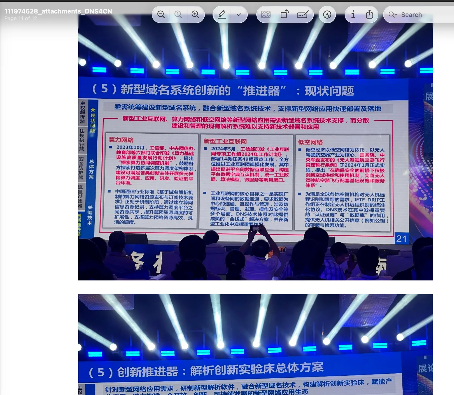
The output is 60 JSONL shards, 617MB of text across 54,761 documents. I also wrote a small utility to manually add documents I discovered later, since no automated pass catches everything. I found the OCR gap by exploring the corpus by hand.

Those shards are the handoff point. Two separate systems read them and never import each other, so I can change one without breaking the other.

Two workflows, two jobs

Batch retrieval answers a question I can already phrase. DNS4CN was a named target with a vocabulary I could enumerate, and triage handled it well.

Triage can’t explore. If I don’t know a term, I can’t search for it, and across a language barrier that covers a lot of ground. So I built the RAG for the fuzzier questions: “what does the corpus say about X,” where X might be phrased in words that never appear in my term lists.

Workflow A: batch retrieval

flowchart TD
    E3[("text/shard_*.jsonl")]
    CFG["config/<topic>.yaml
high / medium / low signal terms"]

    subgraph TRIAGE["Per-topic triage — cheap, re-runnable"]
        S4["Stage 4 · triage
weighted terms, noise caps"]
        S5["Stage 5 · tier 
internal vs external, by path"]
        T3[("tier1 · MESA Lab authored
 28 docs")]
        T4[("tier2 · external research")]
    end

    subgraph RENDER["Slide rendering — local hardware, $0"]
        S6["Stage 6 · rasterize 
PPTX → PNG slides"]
    end

    subgraph ANALYSIS["LLM analysis — Anthropic API"]
        S7["Stage 7 · analyze 
per-doc pass, then synthesis
 $11.81"]
        S8["Stage 8 · translate 
tier1 → English"]
        OUT[("<topic>_findings.md")]
        TR[("translations/*.en.md")]
    end

    CFG --> S4
    E3 --> S4 --> S5
    S5 --> T3
    S5 --> T4
    T3 --> S6
    S6 --> ANALYSIS
    T3 --> ANALYSIS
    S7 --> OUT
    S8 --> TR

    class E3,T3,T4,OUT,TR store
    class S4,S5,S6,S7,S8 stage
    class CFG cfg

Stage 4: rank the documents by topic

Stage 4 is the first cheap filter. I score every document against a topic’s term list: high, medium, and low-signal terms, weighted by hand. The terms live in a per-topic config, so spinning up a new topic takes seconds and never touches the corpus.

The scoring needed noise control, and it needed it because of a spreadsheet. Raw scoring pays 10, 3, and 1 points per occurrence of a high, medium, or low-signal term (respectively). One CSV in the corpus hit DNS 13,948 times, which put a bulk data dump above every piece of real analysis I had. Three filters fixed it: cap how many times low and medium signal terms can count at all (5 and 30), penalize data files that match no high-signal term, and pay a bonus for each distinct term a document matches. That spreadsheet fell from 13,948 to roughly 1.5, while a slide deck matching DNS4CN and 盾立方 and DoH and resolver together climbed. Distinct-term coverage beat raw frequency as a relevance signal.

The output is a ranked list. Nothing here is smart. It’s grep with weights and a scoreboard, and I want it that way: the dumb, auditable step does the culling, so I can see why a document ranked where it did.

Stage 5: split by who wrote it

Scoring tells me a document is about DNS. It can’t tell me who wrote it or why it’s relevant. “Here is a design proposal to block encrypted DNS” and “Here is an IEEE research paper on encrypted DNS” both hit DNS, DoH, and DoT heavily, but only one is a primary source.

So the tier rule combines two signals: a document goes to the internal tier if it matched any high-signal term, or if it sits in one of the internal project directories and carries a Chinese filename. Everything else is external. For DNS4CN that pulled the field down to 28 internal documents worth the expensive read, with the external literature kept as corroboration.

Stages 6–7: rasterize locally, read expensively

Everything up to here ran on hardware I already owned, including Stage 6, where rasterizing slides costs nothing. Stage 7 is the only point in the process where any of this material leaves my machine (and starts creating the expensive calls to Claude Opus).

Stage 6 rasterizes the slide decks. My first pass extracted text from everything, slide decks included, and sent that text to the model. But my extraction had a visibility gap: no rasterization meant the model never saw the diagrams, and missing Chinese fonts had already mangled what text there was.

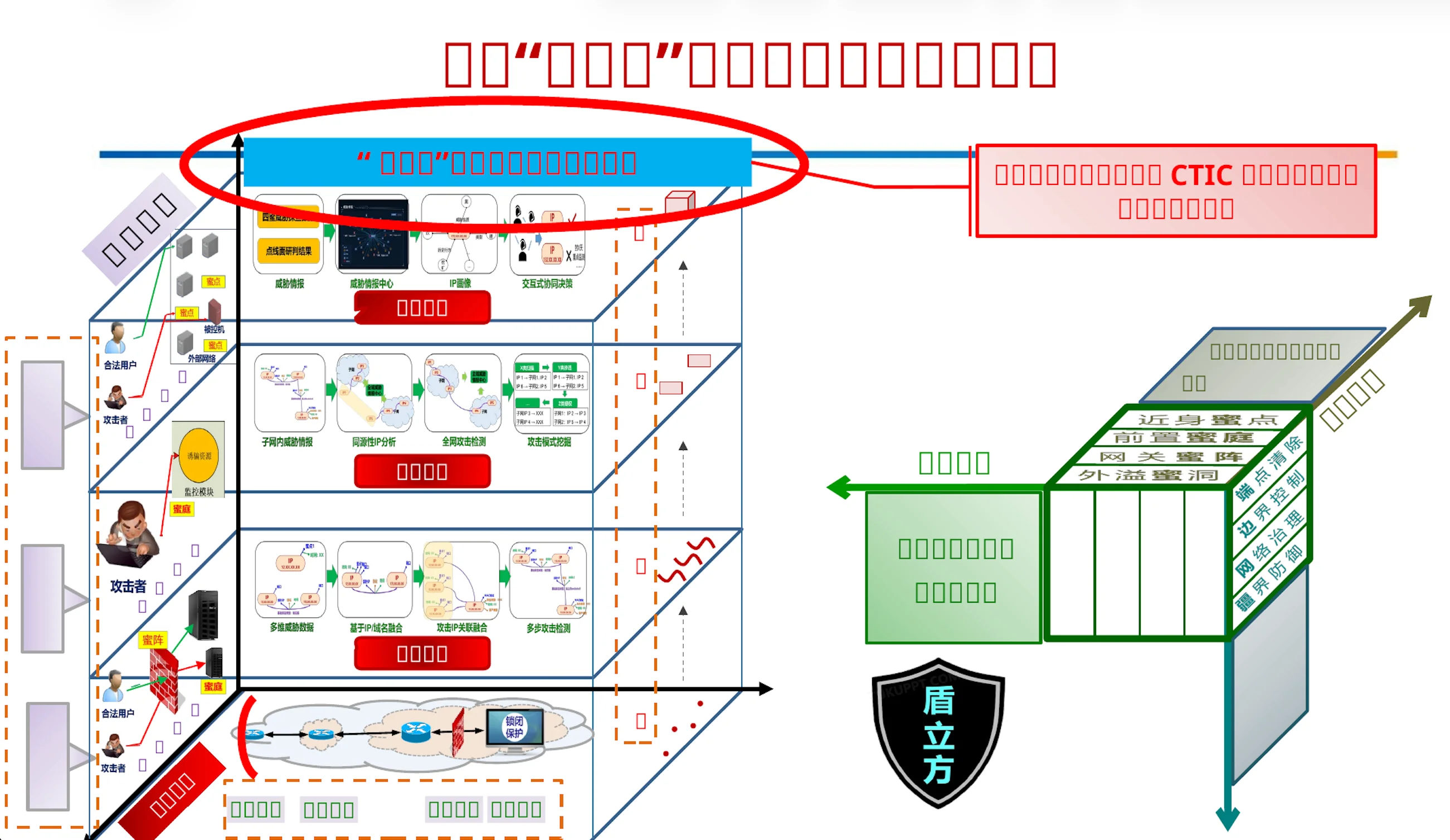
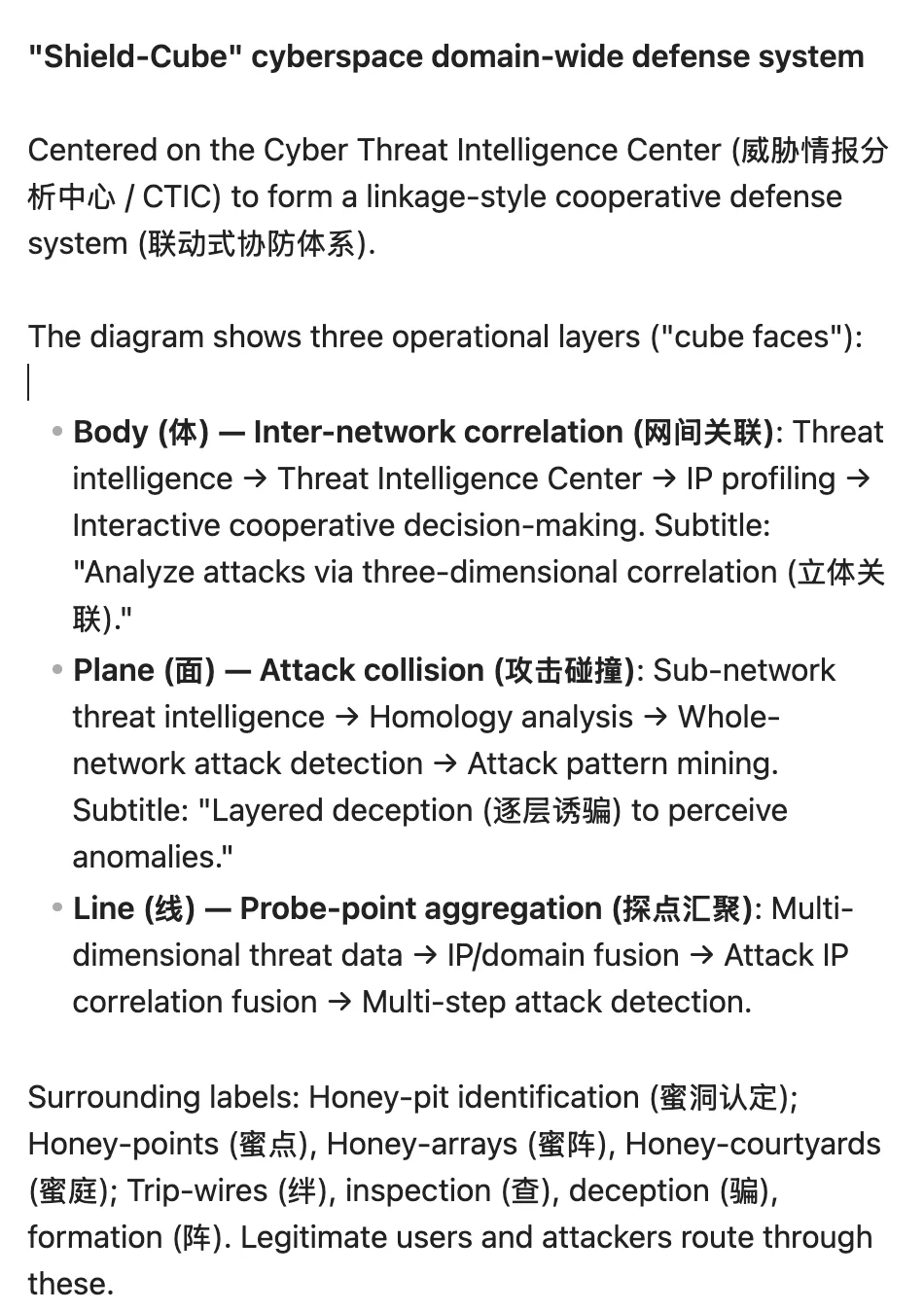
The fix: Stage 6 now rasterizes every tier-one slide deck to PNGs before Stage 7 ever sees it, so the model reads the deck the way a person would. Nearly every figure in the DNS4CN piece came out of this path: architecture diagrams that existed as pictures on slides. Text-only, I would have missed all of it.

Stage 7 - Send to the frontier model It’s two passes. First a per-document read against a fixed schema: what the document claims, who authored it, the mechanism, and evidence quoted in the original Chinese with its file path. Then a synthesis pass across the tier. I don’t write down a finding that can’t produce a file path and an original-language quote.

The synthesis pass rolls the per-document reads into one report: executive summary, architecture and mechanism, every claim still carrying its source filename.

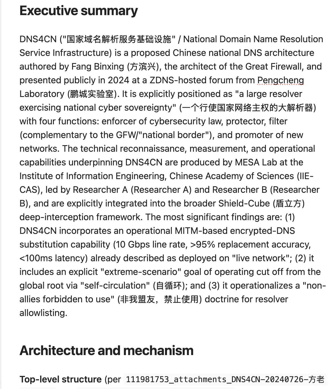
What it actually cost

Four analysis runs over two weeks, plus one translation run:

Run	Docs	Cost
Final analysis run	28	$11.81
Three earlier analysis runs, all superseded	32	$19.74

The final analysis run cost $11.81 for a per-document read of all 28 and one synthesis pass across them. I can’t tell you the exact translation cost. I forgot to record those. My best estimate is around $30 given the remaining balance in my console account. $31.55 + $30 = $61.55 for a topical pass against 55,000 documents (including typos). I think that’s pretty good. But how can I mine this leak for more leads?

Workflow B: the RAG

The RAG is a second system that reads the same 617MB of shards and does its own thing with them. Workflow A ranks whole documents by terms I chose. Workflow B searches meaning, which is the part I couldn’t do by hand in a language I don’t read. The concept is to use the RAG (embeddings) to help create additional keywords for Workflow A.

flowchart TD
    E3[("text/shard_*.jsonl")]

    subgraph INDEX["Index build — one-time, ~1 hr on an RTX 4080"]
        IX["chunk + embed
800 tok / 150 overlap · BGE-M3 fp16"]
        DB[("LanceDB · 14GB
 290,073 chunks")]
    end

    subgraph SEARCH["Query time — interactive, seconds"]
        SE["hybrid search 
dense ⊕ BM25, RRF-fused"]
        Q1["query.py 
 ranked hits + snippets"]
        Q2["ask.py 
 cited answers"]
        Q3["seed_ask.py 
 fixed topic battery"]
    end

    SP["seed_prompts/*.yaml 
grounded schema prompts"]
    OLL["Ollama · gemma4:12b 
local, $0 per query"]
    RPT[("rag/<battery>.md")]

    E3 --> IX --> DB --> SE
    SE --> Q1
    SE --> Q2
    SE --> Q3
    E3 -. re-fetch full text .-> Q2
    SP --> Q3
    Q2 --> OLL
    Q3 --> OLL
    Q3 --> RPT

    class E3,DB,RPT store
    class IX,SE,Q1,Q2,Q3 stage
    class SP cfg
    class OLL ext

Building the index

The index build is a one-time cost. I chunk every document (800 tokens, 150 overlap), embed each chunk with BGE-M3, and store the vectors in LanceDB. That’s 290,073 chunks across the same 54,761 documents, a 14GB index, a few hours on an RTX 4080. After that, searching is interactive and runs in seconds. The index is disposable, rebuildable from the shards whenever I want, which keeps the whole tree portable.

BGE-M3 does the heavy lifting here for one reason: it’s multilingual and trained for retrieval, so a query in English pulls a passage in Chinese when they mean the same thing. That covers the exact gap I have.

Three ways to ask

The same search backs three different scripts. The first returns ranked chunks with snippets, for when I’m exploring and don’t yet have a question. The second answers a single question and forces citations. The third runs a fixed battery of topics through the same grounded schema in one shot, which is what produced the topic reports I worked from. Same retrieval underneath, three levels of “how much do I already know what I’m looking for.” All three answer in English; the evidence quotes stay in the original Chinese.

Same schema, local model

Generation runs on a local Gemma 12B model through Ollama, which means every query costs nothing and no corpus text leaves the box at this stage.

The prompt hands the model the retrieved chunks and a rigid schema to fill: what the document claims, who authored it, the mechanism, foreign models it cites, and evidence quoted in the original Chinese with an English gloss, every quote carrying its source file path. Then a confidence rating and an explicit gaps field. If a claim can’t name a file and quote the original, I don’t keep it.

RAG and False Negatives

Some of my basic prompts returned no findings for a term I knew was in the leak. I’d already read those documents by hand.

In collection terms, “not found” can mean a true absence or a coverage gap, and the system can’t tell me which.

A bad prompt caused this one. Semantic search works by meaning, and some terms don’t have any. An internal project named after a number, or after two ordinary Chinese characters, means something only to the people who named it. The embedder read the characters at face value and retrieved documents about the literal words, crowding out the real material before generation started. Searching the exact string, in Chinese, put the right documents at rank one.

Dense retrieval fails a different way, and this one isn’t the query’s fault. It will rank a near-empty page above real substance, because a stub page embeds as cleanly as a page full of substance.

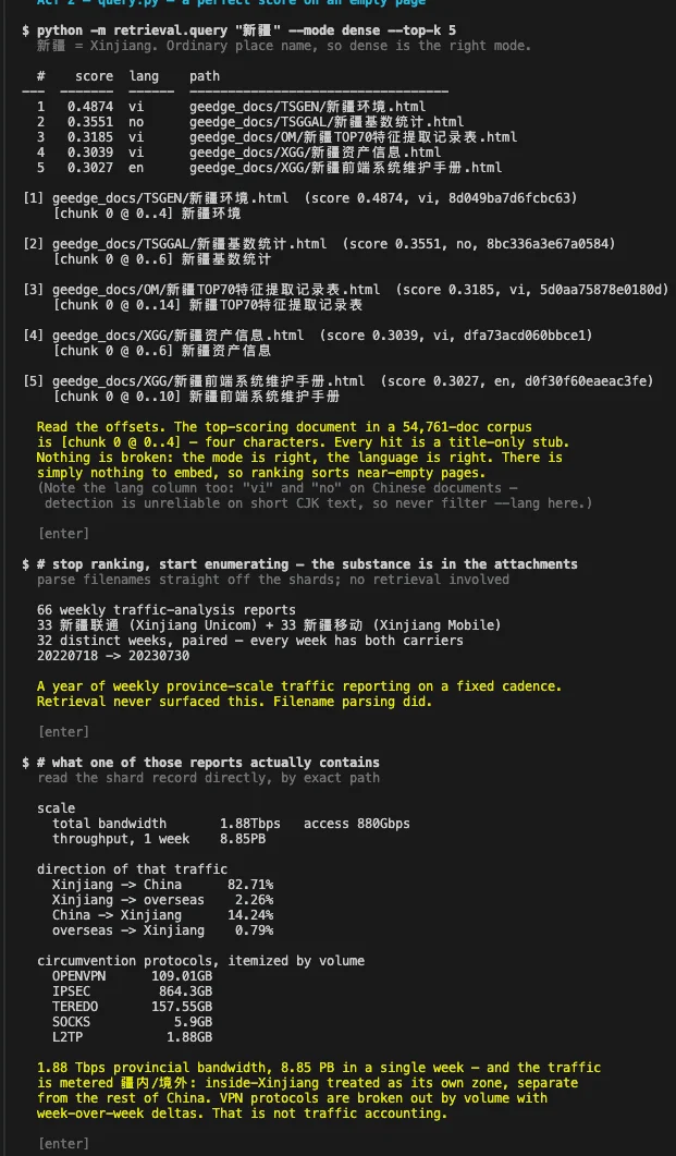
Three things came out of that. Codenames retrieve as exact strings in the source language, and my English translations of them retrieve noise. Filename search found 10 documents carrying the codename; sweeping document bodies found 20, and the most definitional document in the set never mentions it in the title. So before I believe any “not found,” I probe the term’s rank in the index directly, which costs seconds.

Best Practices

What I learned from building this pipeline and researching DNS4CN was pretty straightforward. The expensive part of the pipeline should only see the documents that have already survived the cheap tests. Here are the four biggest lessons I learned.

• Rank the document with methods you can audit, then spend frontier model money on the highest signal ones. The expensive step touched 28 documents and cost $11.81. Fixing all of the bugs along the way, cost another $19.74 in API credits.

• Corroborate the model against a second collection path. The rasterized re-read caught findings the text-only pass got wrong, and the keyword and semantic systems now check each other.

• Force citations everywhere, in the source language. A claim without a file path and an original-language quote does not leave my notes.

• The model earned its place the same way a junior analyst would. It does volume work under supervision, cites its sources, and I check the output by confirming the original Chinese source material. I intentionally built the pipeline so the fact checking stays cheap.

---

Notes and acknowledgements

This post is methodology only. I will not be releasing the source code; however I am releasing redacted (removed researcher names) copies of the major primary source documents on Github. I hope that someone can make use of them or will find them interesting for future reference.

Repo: github.com/jhysler/dns4cn_research